
Our Task
Our task was to predict the NBA draft results of top high school basketball players based on their high school recruiting attributes and college performance. All four project members are close followers of NBA and college basketball and were eager to see what machine learning could tell us about a young prospect’s NBA future. Additionally, we feel that colleges could find an accurate machine learning model useful to help advise their players on the optimal time to enter the NBA draft.
Data Scraping, Cleaning and Preprocessing
We began this project by exploring numerous online basketball data resources. Although the collective amount of information was fairly abundant, we found that no particular source contained all the data we required. Thus, we decided to build a novel dataset from scratch, using the resources listed here. The construction of our dataset required the extensive use of web scraping, scripted data manipulation, and manual data manipulation techniques.
The scraping was completed using multiple software packages which are outlined on our references page. Each resource required an extensive amount of scripting to pull out the exact information we required. After scraping was completed at each stage, the separately pulled datasets needed to be merged with one another, which proved to be the most difficult and time-intensive part of the dataset building process. The merging began with scripted fuzzy and exact string matching, however, significant amounts of manual matching were required to achieve the accuracy we desired for our dataset. This required each group member to carefully parse through and clean data for multiple hours, at each manual cleaning stage.
The final step before plugging our data into the modeling software was preprocessing. The details of this work changed depending on which machine learning technique we were attempting to apply. For example, extensive variable-specific normalization techniques were used to correctly apply the nearest neighbor algorithm to our dataset. Additionally, some attributes were transformed into better proxies for the signals we were considering, such as converting player hometowns to latitudes and longitudes, and bucketing college basketball programs into quality tiers based on our a priori intuition. Lastly, we manually searched and removed those players who were still in college from our dataset and had not yet tried entering the NBA draft.
Data Description
The foundation of our dataset came from the 247Sports Top 100 High School Basketball Recruits Composite Rankings from 2003 to 2017. This allowed us to collect information on players from the earliest possible point, as well as include players who did not attend college at all. In order to significantly reduce noise and maintain a relatively high drafted-to-undrafted ratio, we decided on using only the top 100 recruits (as opposed to the top 200, 500, etc.)
From this starting point we pulled their draft results from an official NBA website and many college performance stats from BasketballReference. In total, our dataset had 62 features, both discrete – position, college, conference – as well as numeric – recruiting ranking/score, height, weight, number of years played in college, longitude/latitude of hometown, and college career and final year stats. In order to practice proper machine learning experimentation, we separated our test set from our training set at the very start, using players in high school classes of 2007, 2009, and 2011 as our test set (a total of 298 examples) and the rest as our training set (a total of 878 examples). See the data section to browse our full dataset and see our full set of attributes. We chose not to include international players and focused solely on American recruits.
Experimental Design
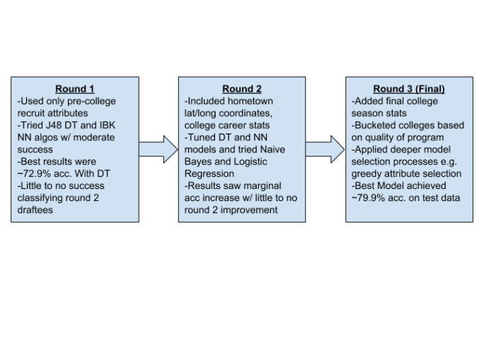
Throughout the project we were constantly trying to build more attributes onto our dataset, test modified/new models, and learn from our results. We iterated through these steps several times, allowing us to gain substantive insights on our project’s main strengths and weaknesses. This process was supplemented by our diligent use of machine learning best practices such as consistently comparing our results against benchmarks like ZeroR and being mindful not to blindly follow model success without any a priori intuition or inductive biases.
We believe that the success of our project can be attributed to our dedication to this thoroughly outlined experimental design. Here is an outline of the details of our iterations and our final experimental results:
Model Selection
While we initially set out to build a machine learning model on all of a recruit’s information (their high school recruiting information and college performance statistics and information), we were also interested in answering a couple more questions: is high school performance or college performance more important in determining draft success, and how telling are the few most important features from our dataset? Furthermore, since we were concerned that we may have included too many noisy attributes and because it was so challenging and time-consuming to scrape and merge all the data we collected from the three different sources, we were intrigued by the idea of only using a subset of the attributes to see if we could build a sufficiently accurate, simpler model for use on our test data.
Full Model
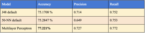
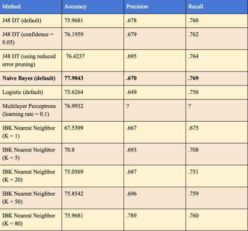
Note: ZeroR achieved 64.9203 % accuracy.
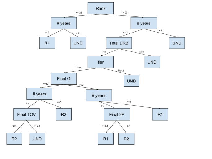
Before applying any intuitive model selection processes, we wanted to naively try several models on all of the attributes we collected. We were aware that including all 62 of our attributes was likely to add a significant amount of noisy and potentially irrelevant information, but we hoped to establish a strong benchmark to improve upon going forward. The Multilayer Perceptron model had the best accuracy, precision, and recall performance out of the models we considered. The power and flexibility inherent in the Multilayer Perceptron algorithm is probably what allowed the model to overcome any noise that was introduced through irrelevant attributes. This result, however, should be taken with a grain of salt, because the size of our dataset makes it very prone to overfitting with such a powerful model. See the table below for more details. Although the decision tree model did not achieve the same level of success, it did provide significant insight into the nature of our dataset and hypothesis space:
Greedy Feature Selection
Secondly, we set out to analyze whether we might be able to build a model with comparable accuracy using just a few of the most important attributes in order to filter out some noise. Thus, we greedily found the four most important attributes by information gain (in order: recruiting rating from high school, number of years played in college, final year assists per game, and final year minutes played). It was interesting to see that rating was the most telling feature, showing that the 247Sports composite ranking may actually be a fine-tuned formula. We were pretty surprised to see that final year assists per game and minutes per game were the third and fourth most telling attribute, as these statistics do not seem to be too indicative of draft success of a player. On the other hand, rebounds and blocks per game (two stats that scouts believe translate well to the NBA style of play) were always very telling attributes in our feature selection process (while not in the top four). After selection, we then tested our dataset with only these 4 features with 10-fold cross validation with different Weka models and some minor settings tuning (see the chart below for the results). Interestingly, our Naive Bayes model proved most accurate in 10-fold cross validation. This may make sense, as the attributes are pretty independent of each other given the draft status (the output class). In summary, it was very interesting to see that using only four attributes, we were able to achieve a higher 10-fold cross validation accuracy than our full dataset. See the table below for details.
College vs High School Attributes
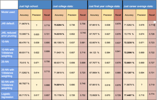
After examining our dataset, it’s clear that our attributes could be split into two categories – a player’s high school recruiting information and their college game statistics. Further, college stats can be broken down into final year and career averages. We thought it would be interesting to explore if one group of these attributes were more predictive than others. The results from these experiments can be seen in the table above. Looking at the results, we see that overall, just college career average stats performed the best across all models (only beaten by decision trees and 50-NN when combined with final year stats). Surprisingly, final year stats alone achieved the lowest results of all the sets tested. Overall, we see that just high school rankings are an adequate predictor, however, the college stats model is much stronger, suggesting that in-game performance is a more important factor when considering draft success.
Results
For our final model, we decided to use the greedy feature selection model. We came to this decision because the full dataset was achieving lower accuracies (due to noisy uninformative attributes), and we preferred it to the just college stats model since it aligns better with our test hypothesis – being able to predict draft outcome based on high school ranking and college statistics – as it contains features from both sets. Furthermore, the four attributes we ended up with are theoretically conditionally independent given the output class as they don’t have really any relation given the draft results of the players. Thus, a Naive Bayes model which relies on this assumption seemed to us like a reputable model to use. Our final test results ultimately confirmed this intuition, and yielded what we consider to be a successful model. The Naive Bayes with Greedy Feature Selection achieved 79.8658% accuracy on our test set of 298 observations from 2007, 2009, and 2011. This translated to an error confidence interval of [15.581%, 24.687%] (using a 95% certainty range). Although the almost-25% error on the high end may seem troublesome, this a statistically significant improvement upon the ZeroR baseline, which yields an error confidence interval of [29.662%, 40.498%].
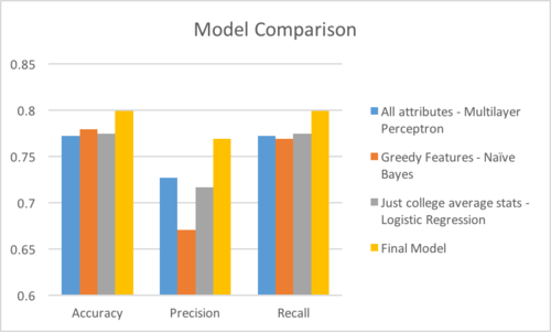
The above graphic shows the accuracy, precision, and recall values of our 3 different tested models, as well as our final model’s performance on the test dataset.
While we showed that our model is statistically significant in its predictions, we realize that the dataset we have used may limit us from getting higher accuracies (e.g. in the 90 percent range). While we did incorporate many attributes about the players in our data set, we realize we are missing substantial information that could improve the models, including accuracy, potential, athleticism, basketball IQ, character, defensive prowess, system fit, and a player passing “the eye test,” all of which are difficult to tease out using statistics alone. In addition, criteria for selection and ranking of players in the draft changes over time. For instance, ten years ago, massive players who could overpower opponents near the rim were highly valued, whereas in recent years, more emphasis has been placed on smaller athletes who can make the three point shot and stretch defenses. As a result, our predicted outcomes likely have an inevitable degree of bias towards old player preferences.
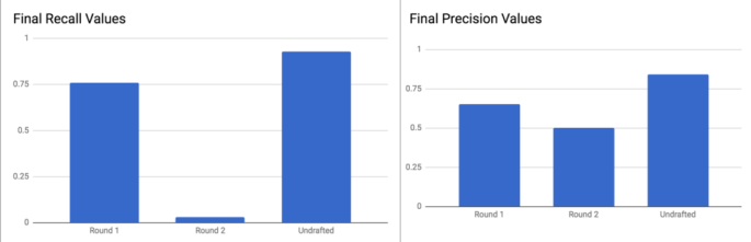
From our test set results we can also take a look at the precision and recall values (see bar graphs below) found from running our test set. We achieved very high values of precision/recall for first round picks and undrafted players, whereas we found extremely low precision/recall extremely low for 2nd round pick. We actually expected these findings and think this is quite normal – in the NBA, once the draft gets past the first round, most teams are drafting players on potential or system fit (two attributes that can’t be quantified), simply hoping to get lucky, as most second round selections fail to even make the team they were drafted by. Thus, we believe that every model we tested throughout our research process achieved low precision and recall values for second round picks because the selection criteria for a second round pick is less clear and less quantifiable in our dataset. As a result, our model only classified two test instances as second round picks.
This academic report has been modified for compatibility with this blog. The original version can be found here.
